When Moonshot AI published Kimi K3 with 2.8 trillion parameters, the reactions split into two camps. Camp one: “2.8T parameters?! This must be the most powerful model ever.” Camp two: “2.8T parameters?! This must be impossible to run.” Both camps are wrong — or more precisely, they’re answering the wrong question.
The 2.8 trillion number is real, but it describes the model’s total parameter count. What actually matters for inference speed and cost is the number of parameters activated per token. In Kimi K3’s case, that’s roughly 50 billion — 56x fewer than the headline number. The model is vast, but any given token only touches a thin slice of it.
That ratio — total parameters vs. active parameters — is the key to understanding every MoE model. Once that clicks, the architecture makes perfect sense.
What Is a Mixture of Experts Model?
A standard (dense) language model like GPT-4 or Claude is dense: every token activates every parameter in the model during inference. When a token flows through a dense transformer layer, it passes through the same weighted computation that every other token passes through. The same experts process every request.
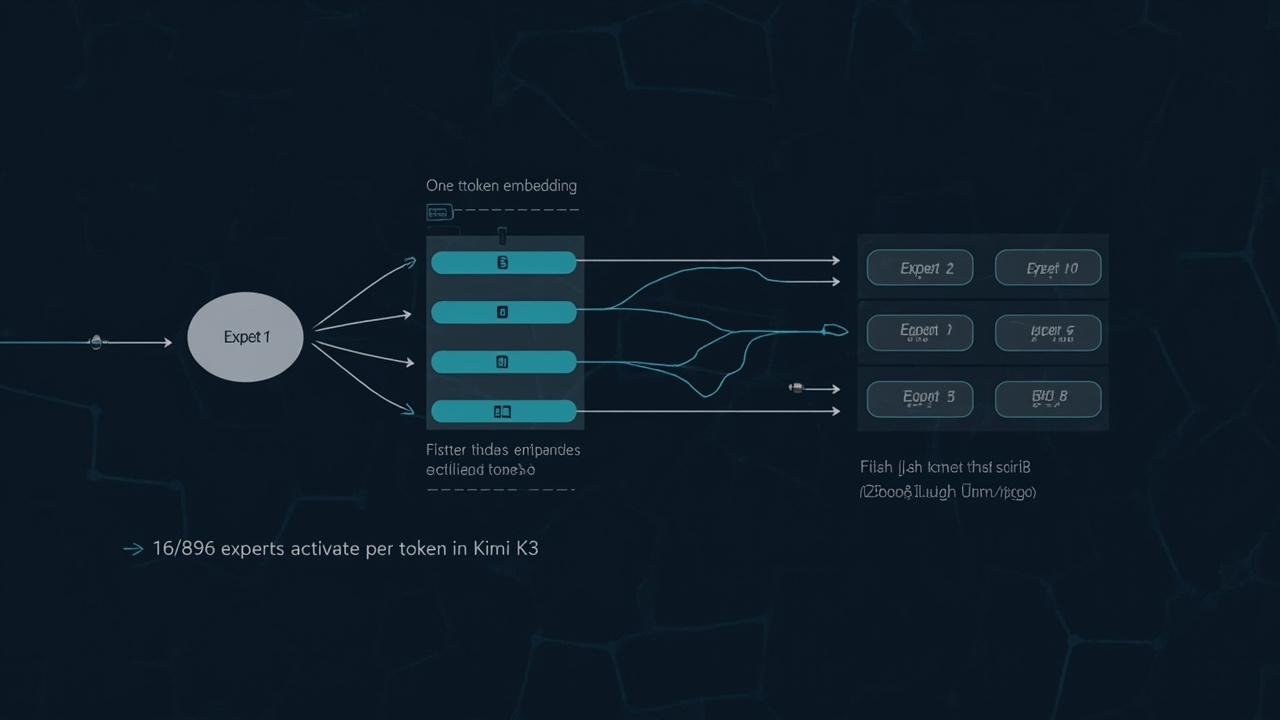
A Mixture of Experts model is sparse: instead of one feed-forward network that everyone shares, there are many specialized experts — each a complete feed-forward neural network with its own weights. A gating network looks at each incoming token and decides: which subset of experts should handle this?
For any given token, only a small number of experts activate. The rest are idle. This means you can have a model with a trillion total parameters but activate only a few billion for each token — the inference cost is determined by the active parameters, not the total count.
Dense model (every token activates all parameters):
Token → [FFN Layer: all weights] → output

MoE model (token activates subset of experts):
Token → [Gating Network] → selects top-K experts → [Only those experts activate] → output
Think of it like a hospital. A general practitioner (dense model) handles every case themselves. A specialist hospital (MoE) has a triage nurse (gating network) who routes each patient to the right specialist. The triage step adds overhead, but each patient gets expert-level attention without requiring every specialist to be involved in every case.
The Three Numbers That Define a MoE Model
Three numbers define any MoE model’s characteristics:
- Total parameters — the sum of all expert weights across the entire model. This is the number that gets reported as the model size. For Kimi K3: 2.8 trillion.
- Active parameters per token — the parameters actually used when processing a single token. This determines inference speed and memory during serving. For Kimi K3: approximately 50 billion equivalent (16/896 experts active).
- Expert count / Top-K — how many experts exist in total, and how many are activated per token. Kimi K3: 896 experts, top-16 active per token.
The sparsity ratio is: total_params / active_params. Kimi K3’s ratio is roughly 2.8T / 50B ≈ 56x. A 2.8T model that behaves like a 50B model during inference. That’s not a bug — that’s the entire point.
The Gating Mechanism: How Experts Get Selected
The gating network is the most important piece of any MoE architecture. It’s a learned router that scores each expert’s relevance to the current token, then selects the top-K experts to handle it.
Token embedding
      ↓
Gating network: scores each expert (learned linear layer → softmax)
      ↓
Top-K selection: pick the K highest-scoring experts
      ↓
Selected experts each process the token in parallel
      ↓
Outputs are weighted and combined
      ↓
Proceed to next layer
In Kimi K3, the gating is part of the Stable LatentMoE framework. The routing happens in latent space rather than directly on token representations, which Moonshot says reduces routing overhead and improves expert utilization.
Why Load Balancing Is the Hard Problem
A gating network that only picks the best expert will develop a positive feedback loop: one expert gets slightly more routing confidence, which means it gets used more, which means it trains more, which means it gets even better scores, which means it gets used even more. The result is that a few experts handle most tokens while others barely train. This is called expert collapse, and it’s the primary failure mode for MoE training.
MoE models solve this with load balancing constraints. The original Switch Transformer (Google, 2021) introduced an auxiliary load-balancing loss that penalizes models for over-relying on any single expert. Mixtral (Mistral, 2023) used auxiliary load-balancing with auxiliary load terms in the loss function.
Kimi K3’s Stable LatentMoE takes a different approach with Quantile Balancing: instead of using a heuristic update rule for expert allocation (which introduces a sensitive hyperparameter to tune), Quantile Balancing derives expert allocation directly from router-score quantiles. This makes expert utilization more stable during training at the 2.8-trillion-parameter scale.
MoE vs Dense: A Concrete Comparison
The comparison that makes MoE click:
| Characteristic | Dense Model | MoE Model (Kimi K3) |
|---|---|---|
| Total parameters | 70B | 2.8T |
| Activated per token | 70B | ~50B |
| Inference cost | 70B FLOPs/token | ~50B FLOPs/token |
| Memory for weights | 140GB (FP16) | 5.6TB raw → ~700GB (MXFP4) |
| Expert structure | 1 FFN | 896 experts, 16 active |
| Routing overhead | None | Gating + load balancing |
The dense model activates all 70B parameters every token. Kimi K3 activates ~50B — a similar cost profile to a 50B dense model, but with 56x more total parameters in the model. You get the capacity of a 2.8T model (which translates to better performance on complex tasks) at the inference cost of a 50B model.
Kimi K3: The Architecture Details
Kimi K3 is the first open model to hit the 3-trillion-parameter class. But the architecture is where it gets interesting. Three major innovations:
1. Kimi Delta Attention (KDA)
Standard transformer attention has quadratic complexity — the attention cost grows with the square of the sequence length. For a 1-million-token context window, this is prohibitively expensive.
KDA replaces standard quadratic attention in a subset of layers with a hybrid linear attention mechanism. It maintains full expressiveness for critical layers while dramatically reducing the compute cost of attention across long sequences. This is what makes the 1M-token context window feasible at inference.
2. Attention Residuals (AttnRes)
Standard residual connections (output = input + layer(input)) accumulate layer outputs uniformly — each layer contributes equally to the final representation, regardless of whether earlier layers had relevant information.
AttnRes allows each layer to selectively retrieve representations from arbitrary earlier layers rather than accumulating them uniformly. In an MoE architecture where different experts activate at different depths, this matters: a layer can reach back directly to the expert output from an earlier layer that specialized in a relevant pattern, without waiting for it to propagate through every intermediate layer.
3. Stable LatentMoE
This is the MoE framework managing 896 experts with 16 active per token. Key engineering challenges:
- Latent-space routing: Instead of routing on raw token representations (which can be noisy), Stable LatentMoE routes in a learned latent space where expert assignments are more stable
- Quantile Balancing: Load balancing derived from router-score quantiles, avoiding the sensitive hyperparameter in prior auxiliary-loss approaches
- Per-Head Muon: Muon is a gradient descent variant; Per-Head Muon extends it by optimizing attention heads independently for more adaptive learning at scale
MXFP4 Quantization: How 2.8T Parameters Fit in Memory
The raw FP16 weights for 2.8T parameters would be 5.6 TB. That’s not practical. Kimi K3 uses MXFP4 (Microscaling FP4) — a quantization format that’s central to making the model deployable.
MXFP4 is an open standard from the OCP MX Formats specification. Unlike standard INT4 quantization (which quantizes to 4-bit integers), MXFP4 is 4-bit floating point with per-block scaling factors. A group of values share a single scale factor, which lets the format preserve more precision where model weights concentrate.
The practical effect: MXFP4 enables roughly 4x compression vs FP16 while maintaining accuracy that approaches full FP16. MXFP4 weights with MXFP8 activations give broad hardware compatibility — it’s supported on AMD MI300X and NVIDIA Hopper (H100/H200).
The training approach also matters: Kimi K3 applies quantization-aware training (QAT) from the supervised fine-tuning stage, not post-training quantization. The model learns to compensate for quantization error during training, resulting in significantly less quality degradation than quantizing a fully-trained model.
The Benchmark Numbers
Kimi K3’s benchmark profile:
| Benchmark | Score | Notes |
|---|---|---|
| GPQA Diamond | 93.5% | Graduate-level science reasoning |
| AIME 2026 | 94.5% | Math competition |
| SWE-bench Verified | ~87% | Real software engineering tasks |
| Terminal-Bench 2.1 | 88.3 | CLI task completion |
| DeepSWE | 67.5 | DeepSeek’s coding benchmark |
For context: Claude Opus 4.7 hits ~83.5% on SWE-bench Pro. Kimi K3’s numbers put it in the top-tier on coding and reasoning benchmarks. On GPQA Diamond (graduate-level science), it’s at 93.5% — ahead of most other open models.
The always-on thinking mode (similar to extended thinking on Claude/GPT) is on by default, which contributes to these scores. The model reasons step-by-step before producing its final answer.
How to Run Kimi K3
Weights were released July 27, 2026 — freely downloadable. Here’s the practical reality:
The Hardware Math
The raw numbers: 2.8T parameters at FP16 = 5.6 TB of weights. No single GPU can hold this.
With MXFP4: approximately 700 GB. Still requires multiple GPUs or specialized hardware.
With llama.cpp / GGUF: Kimi K2.6 (the predecessor) quantized to Q4_K_M fits in ~200GB, which fits on a high-end workstation with enough RAM or a multi-GPU setup.
For the full model at reasonable speed, the realistic options:
| Setup | Feasibility |
|---|---|
| Consumer GPU (RTX 4090 24GB) | Not feasible — needs ~29x that |
| High-end workstation (512GB RAM) | Marginal — MXFP4 or aggressive Q4 |
| 1x H100 80GB | Marginal — needs ~9x that |
| 8x H100 80GB SXM | Feasible — vLLM supports this config |
| Cloud API (Kimi Platform) | Most practical today |
Running via API (Practical Today)
# Via Kimi Platform API
curl https://api.moonshot.ai/v1/chat/completions \
  -H "Authorization: Bearer $MOONSHOT_API_KEY" \
  -H "Content-Type: application/json" \
  -d '{
    "model": "kimi-k3",
    "messages": [{"role": "user", "content": "Explain MoE architecture"}],
    "temperature": 0.3
  }'
Pricing: $3 / 1M input tokens, $15 / 1M output tokens (thinking mode included).
Running Locally (Weights Released)
The vLLM team is actively preparing Kimi K3 support (announced July 22, 2026). The expected path:
# Once vLLM support lands and weights are on HuggingFace:
vllm serve moonshotai/Kimi-K3 \
  --tensor-parallel-size 8 \
  --quantization mxfp4
Unsloth has published guides for running Kimi K2.6 locally with llama.cpp and GGUF quantization. The K3 weight release will follow a similar pattern: first the community quantizes down to Q4/Q5, then llama.cpp/ollama support lands, then it becomes accessible on consumer hardware.
For now, Kimi K2.6 (the predecessor) is the more practical local target — it fits on a 256GB workstation with aggressive quantization and demonstrates most of the architectural innovations.
Ollama (Easiest Path)
Ollama added Kimi K2 support in July 2026 with a cloud sync option:
# Cloud option — no local GPU needed
ollama run kimi/k2.6:cloud

# Local (once K3 weights and Ollama support land)
ollama run kimi/k3
Ollama’s cloud mode streams the inference to Moonshot’s API with your local Ollama client handling the interaction — useful if you want the local tooling experience without local inference hardware.
Why the MoE Moment Matters
The 2.8T parameter count is a milestone, but the real story is architectural. Kimi K3 proves that:
- Open models can hit the frontier — 93.5% on GPQA, 87%+ on SWE-bench, 94.5% on AIME puts K3 in the top tier alongside proprietary models
- Scaling doesn’t have to mean proportional inference cost — the MoE architecture means you get a 2.8T model at ~50B inference cost
- Open weights at this scale changes the research landscape — quantization studies, fine-tuning experiments, inference optimization work, and architecture research all become possible on the same model class that powers frontier API services
The MoE architecture has been the dominant design for frontier models since GPT-4 (rumored) and Mixtral (confirmed, 2023). With K3’s open release, the research community gets direct access to the architecture that powers the current frontier — not a reference implementation, but a production-scale model.
Whether you run it via API, deploy it with vLLM on a GPU cluster, or wait for consumer-grade quantization to land, the model is worth understanding at the architectural level. The expert routing, the load balancing, the quantization — these are the primitives that make models at this scale work, and they’ll show up in the next generation of open models too.
Links: Kimi K3 Technical Blog · HuggingFace Model Overview · vLLM K3 Preview · Kimi K3 on OpenLM · Unsloth K2.6 Local Guide
Comments
Powered by GitHub Discussions via Giscus. Sign in with GitHub to leave a comment.